Preface

Scientific Framing of the Report

SOCCR2’s focus areas and guiding questions were inspired by the community-led report entitled A U.S. Carbon Cycle Science Plan (Michalak et al., 2011), whose goals and emphasis include global-scale research on long-lived, carbon-based greenhouse gases (GHGs), mainly carbon dioxide (CO₂) and methane (CH₄)⁴, and the major pools and fluxes of the global carbon cycle. Further bolstering the science plan goals, SOCCR2 has a greater emphasis on the United States and North America within a global context:

1. How have natural processes and human actions affected the global carbon cycle on land, in the atmosphere, in the ocean and other aquatic systems, and at ecosystem interfaces (e.g., coastal, wetland, and urban-rural)?

2. How have socioeconomic trends affected atmospheric levels of the primary carbon-containing gases, CO₂ and CH₄?

3. How have species, ecosystems, natural resources, and human systems been impacted by increasing GHG concentrations, associated changes in climate, and carbon management decisions and practices?

Note that U.S. federal GHG inventories are the responsibilities of several federal agencies. SOCCR2 does not seek to evaluate, critique, or validate those inventories but rather to explore and present the current state of the science of the carbon cycle. Any discussions of current U.S. GHG inventories are conducted within the broader context of the carbon cycle. Where there are any apparent discrepancies with U.S. GHG inventories, or where otherwise appropriate, SOCCR2 explains or identifies the different sources of the discrepancies.

Framing of Report

SOCCR2 is framed around the following topics:

1. Global Carbon Cycle Overview—Major elements of the global carbon cycle (e.g., CO₂ and CH₄,) and key interactions with climate forcing and feedback components from a global perspective (see Box P.2, Global Carbon Cycle, Global Warming Potential, and Carbon Dioxide Equivalent).

2. Carbon Cycle at Scales—Assessment of the North American carbon cycle (scaled down from the global system), including short- to long-term and local, regional, and national perspectives on key carbon stocks and fluxes.

3. Carbon in Unmanaged and Managed Systems—Estimates and assessment of major carbon stocks and fluxes within and among pools, key uncertainties, social drivers, and effects of past management decisions. Example focus areas include:

   • Urban and human settlements;

   • Livestock and wildlife;

   • Soils;

   • Aquatic systems; and

   • Vegetation.

4. Interactions and Disturbance Impacts to the Carbon Cycle—Role of disturbances on the carbon cycle, for example:

   • Fires;

   • Ocean acidification;

   • Pests and diseases of ecosystem components; and

   • Land-use change and land-cover change.

5. Carbon Cycle Management Practices, Tools, and Needs at Various Scales:

   • Role of recent carbon management practices;

   • Current state of carbon data management;

   • Monitoring systems;

   • Tools;

   • Carbon-relevant modeling scenarios; and

   • Mitigation.

Author Guidance and Chapter Organization

To ensure consistency throughout SOCCR2 with regard to methods, approaches, and considerations of scientific quality, an author guidance document was developed, in consultation with USGCRP, by the SOCCR2 planning team (Federal Steering Committee, the U.S. Carbon Program Office, and Science Leads), along with the ORNL technical editing team. Formal guidance on Information Quality was also provided (see Appendix B: Information Quality in the Assessment). The author guidance established a recommended methodology and chapter structure (including templates) for composing the chapters as described below. In some cases, the chapter structure or template was modified by the authors, as appropriate, based on a chapter’s specific relevance to the structure and information type (e.g., Ch. 6: Social Science Perspectives on Carbon).

1. Introduction—Summarizes the topic of the chapter, specifying the key questions needed to understand and quantify the carbon cycle. Spatial and temporal scales relevant to the chapter are described.

2. Historical Context—Summarizes the history of carbon stock and flux quantification with regard to the spatiotemporal scope of the chapter. Historical context includes socioeconomic drivers of carbon emissions (where appropriate), along with an introduction to the use of different approaches and their evolution over time, particularly focusing on findings that have emerged since SOCCR1 (CCSP 2007).

3. Current Understanding of Carbon Fluxes and Stocks—Discusses the “state of the science” in terms of conceptually understanding, measuring, quantifying, and modeling the carbon cycle at the spatiotemporal scale of the chapter. As appropriate, this section describes different methodologies used in research activities and mentions the various assumptions and caveats for each approach (see Appendix C: Selected Carbon Cycle Research Observations and Measurement Programs).

4. Indicators, Trends, and Feedbacks—Describes the exact observed indicators and trends of the carbon cycle at the spatiotemporal scale of the chapter. This includes understanding of the extent of agreement or disagreement between presumed trends, pre- and post-2007 (if applicable). The section also summarizes feedbacks among different ecosystem compartments or pools of Earth System Models or process models. Feedbacks to one ecosystem compartment may provide critical input to another compartment, for example, or from one spatial scale to another.

5. Global, North American, and Regional Context

   • National Climate Assessment (NCA) 2014 and 2018 regions—Places carbon processes, stocks, and fluxes at a particular scale in the chapter in the context of NCA regions, which are reflective of the scale at which physical and environmental processes operate. NCA regions also could be considered “actionable” by policymakers. The NCA 2014 regions consist of Northeast, Southeast, Midwest, Great Plains, Southwest, Northwest, Alaska, Hawai’i, and United States–Affiliated Pacific Islands, Rural Communities, and Coasts. NCA 2018 splits the Great Plains region into the Northern Great Plains and Southern Great Plains and divides the Caribbean and Southeast into separate regions.

   • United States, Mexico, and Canada—Places carbon processes, stocks, and fluxes at a particular scale in the chapter in the context of North America and the planet, scales at which most Earth System Models operate. When available, country-level information also is presented because it is at a scale that policymakers could consider actionable.

6. Societal Drivers, Impacts, and Carbon Management Decisions—Focuses on observed and projected impacts of changes in or to the carbon cycle for the ecosystems being considered. Also described are societal costs of the impacts, including economics. Information about carbon management decisions is intended to summarize the impacts of past decisions (if applicable), evaluate the efficacy of those decisions regarding their intended consequence, and highlight techniques for determining the effects of decisions on the targeted system. The section also could pose relevant scientifically based carbon management concepts as summarized from the literature.

7. Synthesis, Knowledge Gaps, and Outlook—Provides an overarching synthesis of the current state of the carbon cycle, describes knowledge gaps and opportunities, and discusses the near-term future outlook of the North American carbon cycle. Although the goal of SOCCR2 is to highlight and synthesize the current state of the science on carbon cycling in North America, the research needs and critical scientific gaps identified through the development of each chapter and described in this section may serve to inform ongoing and future studies by the scientific community.

Geographical Scope

The major focus of SOCCR2 is North America, with an emphasis on the United States. This emphasis is consistent with the report’s purpose of providing solid scientific information to 1) U.S. decision makers and policymakers that could be used to formulate activities or policies, 2) the scientific community, and 3) teachers for educational use in the classroom. Because the effects of carbon cycle changes are global-scale issues, SOCCR2 addresses carbon cycling from a global perspective, where appropriate. Moreover, since SOCCR2 seeks to be consistent with SOCCR1 (CCSP 2007), which focused on North America, chapters also consider the carbon cycle in Canada and Mexico. Regional-scale discussions may be included where appropriate. The geographical scope of U.S. analysis for SOCCR2 includes the conterminous United States, Alaska, Hawai’i, and Puerto Rico. U.S. regional studies, if included, are presented where processes and impacts vary significantly across the nation and where regional information is available (see Figure ES.1 in the Executive Summary).

Time Frames

Assessing the balance of respective sources and sinks within the Earth system and the atmosphere is complicated by many factors. Exchanges of carbon among different reservoirs can occur in different time frames, with some reservoirs having very dynamic fluxes and responding almost instantaneously to change and other reservoirs having fluxes that are driven by controls that work on much longer timescales of decades to centuries. SOCCR2 is focused on a time frame relevant to understanding and predicting the carbon cycle and the effects of changes to the carbon cycle now and into the near future. The U.S. Global Change Research Act of 1990 mandates a scope of 25 years and 100 years from present day. As appropriate, SOCCR2 describes the relevant timescales, with retrospective estimates mostly representing the decade since SOCCR1 (i.e., 2004 to 2013) and projections involving time frames of decades to a century.

The emphasis is on presenting the scientific understanding and developments that have emerged in the last decade since SOCCR1 (CCSP 2007), which covered the science through 2005. The historical context may go farther back, as appropriate, considering the data sources and the need to set the historical context. Model simulations may begin with preindustrial or geological time frames to converge with current estimations of carbon stocks or concentrations and landscape configuration, for example. For literature data and reviews, the time frame may vary depending on the focus of the relevant literature or model simulations. Chapters or sections describing the impacts of changes to the carbon cycle, mitigation plans, or adaptive strategies also may pose future scenarios.

SOCCR2 summarizes the latest science in North America, using time frames that may differ from ones used for inventories (e.g., U.S. EPA Inventory). For example, inventories are updated regularly, and scenarios used in analyses and related to the policies and politics of climate change and GHG emissions are rapidly changing. On the other hand, research investigations to understand and explain fluxes and changes in both ecological and social contexts often take many years. Time frames also were based on the latest available and comparable carbon cycle data for all three SOCCR2 countries when assessed together. For instance, Ch. 8: Observations of Atmospheric Carbon Dioxide and Methane, selected the Carbon Dioxide Information Analysis Center (CDIAC) time series to represent fossil fuel emissions from Canada, the United States, and Mexico from 2004 to 2013 because of CDIAC’s long historical coverage for all three countries for that time frame and for the clear definition of what goes into the country totals (Marland et al., 2007).

Complex Linkages and the Role of Non-Climate Stressors

Multiple factors, including climate, may exacerbate or moderate the impact of changes to the carbon cycle on ecosystems, processes, and society, as well as potential feedbacks from these changes to the climate system. For example, the history of land-use change, natural climate variability, landscape-scale heterogeneity, anthropogenic effects, and more may affect an ecosystem’s vulnerability to carbon cycle changes and the vulnerability of its carbon pools to changes in climate. Many of these complex interactions and cascading effects are not well understood and thus not entirely addressed in SOCCR2.

Frameworks for Carbon Accounting

Two approaches to quantify carbon cycle components inform research and analysis for scientific studies, and for management and decisions: “production-based” and “consumption-based” accounting. These approaches provide different insights and inform different stakeholder interests and management decisions. To satisfy the requirement for numerical coherence throughout analyses of the carbon cycle in North America, SOCCR2 predominantly uses a production-oriented approach. The production-based or “in-boundary” accounting considers flows of CO₂ and CH₄ into and out of specific areas of land or water. For a hectare of land, net emissions result from, for example, photosynthesis, absorption of CO₂ by concrete, combustion of fossil fuel at a power plant, and the decay of plants and animals on that parcel. In practice, analyses of terrestrial ecosystems such as forests and grasslands also typically include lateral transfers of carbon among parcels (e.g., via erosion or streamflow). The other accounting approach, consumption-based accounting, assigns carbon flows associated with products and services (e.g., timber, electricity, food, chairs, televisions, and heat) to the places where people ultimately use those products. This approach captures demand and trade as drivers of carbon emissions. Emissions from fossil fuel combustion to produce electricity are assigned not to a power plant but to the places where people use that electricity; emissions from crop production are assigned to the place where food is consumed (by humans or animals); carbon captured in trees harvested for timber is assigned to the timber mill or to the place where the timber is used. Quantification of these indirect fluxes typically uses a life cycle assessment framework and also can quantify the carbon stock residing in infrastructure and materials. See Appendix D: Carbon Measurement Approaches and Accounting Frameworks for a more complete description of carbon accounting approaches and their implications.

Methods for Estimating Carbon Stocks and Fluxes

The SOCCR2 author teams assessed research findings based on three observational, analytical, and modeling methods to estimate carbon stocks and fluxes: 1) inventory measurements or “bottom-up” methods, 2) atmospheric measurements or “top-down” methods, and 3) ecosystem models (see Appendix D for details). “Bottom-up” estimates of carbon exchange with the atmosphere depend on measurements of carbon contained in biomass, soils, and water, as well as measurements of CO₂ and CH₄ exchange among the land, water, and atmosphere. Examples include direct measurement of power plant carbon emissions; remote-sensing and field measurements repeated over time to estimate changes in ecosystem stocks; measurements of the amount of carbon gases emitted from land and water ecosystems to the atmosphere (in chambers or, at larger scales, using sensors on towers); and combined urban demographic and activity data (e.g., population and building floor areas) with “emissions factors” to estimate the amount of CO₂ released per unit of activity.

Top-down approaches infer fluxes from the terrestrial land surface and ocean by coupling atmospheric gas measurements (using air sampling instruments on the ground, towers, buildings, balloons, and aircraft or remote sensors on satellites) with carbon isotope methods, tracer techniques, and simulations of how these gases move in the atmosphere. The network of GHG measurements, types of measurement techniques, and diversity of gases measured has grown exponentially since SOCCR1 (CCSP 2007), providing improved estimates of CO₂ and CH₄ emissions and increased temporal resolution at regional to local scales across North America.

Ecosystem models are used to estimate carbon stocks and fluxes with mathematical representations of essential processes, such as photosynthesis and respiration, and how these processes respond to external factors, such as temperature, precipitation, solar radiation, and water movement. Models also are used with top-down atmospheric measurements to attribute observed GHG fluxes to specific terrestrial or ocean features or locations.

Treatment of Uncertainty in SOCCR2

Uncertainty in estimates of values in this report is based on standards established in SOCCR1 (CCSP 2007) and NCA3 (Melillo et al., 2014). The notations and definitions of uncertainty described in this section pertain primarily to reported estimates of carbon stocks and fluxes that are based on statistical sampling or other analytical approaches for which uncertainty can be quantitatively or qualitatively assessed.

In many (if not most) cases, a quantitative statistical uncertainty estimate does not exist for all available numerical values from the literature, so deducing the level of uncertainty using an expert opinion approach is necessary. If quantitative uncertainty estimates are not available, reported uncertainty levels are based on the expert assessment and consensus of the author team. The authors determine the appropriate level of uncertainty by assessing the available literature, determining the quality and quantity of available evidence, and evaluating the level of agreement across different studies. When the underlying studies provide their own estimates of uncertainty and confidence intervals, these confidence intervals are assessed by the authors in making their own expert judgments. A range of estimates may be presented in cases where there are multiple estimates available from different sources or methodologies. For example, estimating the magnitude of the North American terrestrial carbon sink is possible using several approaches: compiled inventories, atmospheric inversions, or modeling that may be informed by remote sensing. It is not practical to quantitatively estimate uncertainty when combining such estimates to derive a single value, in which case a single value may be estimated using expert opinion, or a range of values without also showing a quantitative uncertainty estimate.

Estimating Ranges of Quantitative Values

Unless otherwise noted, values presented as “y ± x” should be interpreted to signify that the authors are 95% confident that the actual value is between y – x and y + x. The 95% boundary was chosen to communicate the high degree of certainty that the actual value is in the reported range and the low likelihood (5%) that it is outside that range. This range may reflect a statistical property of the estimate or, more likely, expert judgment based on all known published descriptions of uncertainty surrounding the “best available” or “most likely” estimate.

Uncertainty of Numerical Estimates

In many tables and figures, a series of asterisks is used to express the uncertainty of numerical estimates (which may be based on statistical properties or expert judgment):

1. ***** — Very high confidence (95% certain that the actual value is within 10% of the estimate reported).

2. **** — High confidence (95% certain that the actual value is within 25% of the estimate reported).

3. *** — Medium confidence (95% certain that the actual value is within 50% of the estimate reported).

4. ** — Low confidence (95% certain that the actual value is within 100% of the estimate reported).

5. * — Very low confidence (uncertainty greater than 100%).

Key Findings and Supporting Evidence

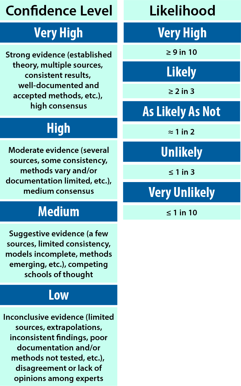
Each chapter includes Key Findings based on the authors’ consensus expert judgment of the assessed scientific literature. Each Key Finding is accompanied by a Supporting Evidence section, which includes each Key Finding’s “Traceable Account” description. This section and the traceable account 1) provide additional information to readers about the quality of the information used, 2) allow traceability to resources and data, 3) document the process and rationale the authors used in reaching the conclusions in a Key Finding, and 4) describe the confidence level and likelihood in the Key Finding, as appropriate (see Figure P.2, this page). For each Key Finding, authors characterize confidence levels quantitatively when possible, and, when not possible, they rank uncertainty qualitatively by reporting their level of confidence in the results.