<b>Gurney</b>, K. R., P. <b>Romero-Lankao</b>, S. <b>Pincetl</b>, M. Betsill, M. Chester, F. Creutzig, K. Davis, R. Duren, G. Franco, S. Hughes, L. R. Hutyra, C. Kennedy, R. Krueger, P. J. Marcotullio, D. Pataki, D. Sailor, and K. V. R. Schäfer, 2018: Chapter 4: Understanding urban carbon fluxes. In Second State of the Carbon Cycle Report (SOCCR2): A Sustained Assessment Report [Cavallaro, N., G. Shrestha, R. Birdsey, M. A. Mayes, R. G. Najjar, S. C. Reed, P. Romero-Lankao, and Z. Zhu (eds.)]. U.S. Global Change Research Program, Washington, DC, USA, pp. 189-228, https://doi.org/10.7930/SOCCR2.2018.Ch4.
Understanding Urban Carbon Fluxes
4.2.1 Accounting Framework and Methods
Many urban researchers, using a spectrum of methodological frameworks and measurement approaches, have quantified urban carbon flows and stocks in North American cities. The accounting framework determines the meaning and application of urban carbon flux information. Broadly speaking, two frameworks have been used: accounting for direct fluxes only or accounting that also includes indirect fluxes occurring outside the chosen urban area but driven by activities within it (Gurney 2014; Ibrahim et al., 2012; Wright et al., 2011). The former, also variously referred to as “production-based” or “in-boundary” accounting, quantifies all direct carbon flux between the Earth’s surface and the atmosphere within the geographic boundaries of the urban area of study (Chavez and Ramaswami 2011; Ramaswami and Chavez 2013; Wright et al., 2011). In-boundary accounting also is aligned with “scope 1” flux, a term emanating from carbon footprinting of manufacturing supply chains (WRI/WBCSD 2004). This framework will include within-city combustion of fossil fuels, exchange of carbon with vegetation and soils, absorption by concrete, human respiration, anaerobic decomposition, and CH4 leaks. An in-boundary accounting framework often is favored for integration with atmospheric measurements, which also can be used to estimate surface-to-atmosphere fluxes within the chosen geographical domain (Lauvaux et al., 2016).
Indirect fluxes include those associated with energy used to create or deliver electricity, products, or services consumed in a given urban area or the carbon flux associated with waste decay or removal of material to the waste stream (Minx et al., 2009; Mohareb and Kennedy 2012). These fluxes include consumption-based flow of products manufactured outside the consuming city (see Figure 4.3). A study of eight cities found that the urban carbon footprint increased by an average of 47% when indirect fluxes were included (Hillman and Ramaswami 2010). Quantification of indirect fluxes typically employs a life cycle assessment framework and also can quantify the carbon stock residing in urban infrastructure or materials (Churkina et al., 2010; Fraser and Chester 2016; Hammond and Jones 2008; Lenzen 2014; Reyna and Chester 2015).
Figure 4.3: Relationships Between Carbon Inventory Approaches.
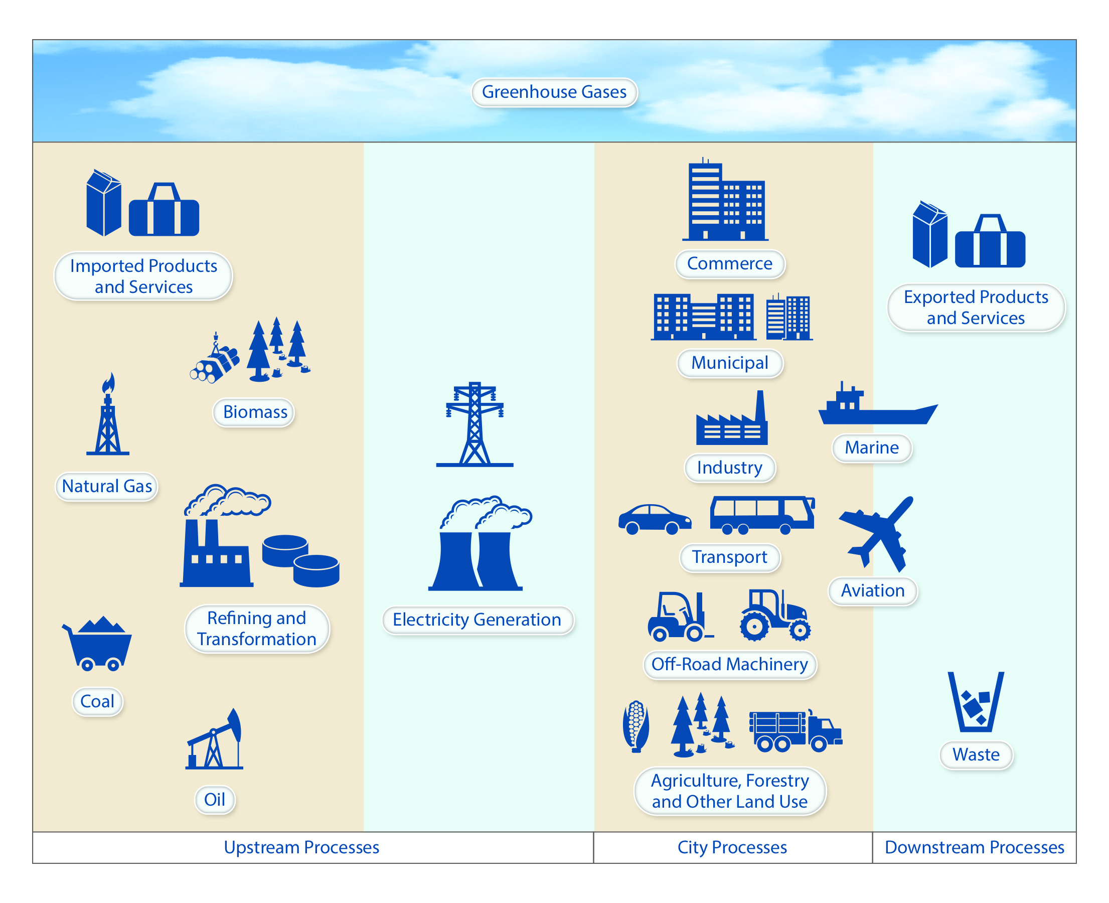
In practice, urban carbon flux studies have used hybrids of the two frameworks, and the mixture reflects academic disciplinary interest, practical policy needs, and differing notions of responsibility or environmental justice (Blackhurst et al., 2011; Lin et al., 2015). There have been important attempts at standardizing urban carbon flux accounting frameworks via protocols or Intergovernmental Panel on Climate Change (IPCC)–approved methods (Carney and Shackley 2009; Ewing-Thiel and Manarolla 2011; Fong et al., 2014; WRI/WBCSD 2004). However, comparing urban carbon fluxes remains challenging without careful consideration of the accounting framework, city boundaries, and flux categories (Bader and Bleischwitz 2009; Hsu et al., 2016; Kennedy et al., 2009; Lamb et al., 2016; Parshall et al., 2010).
Distinct from the accounting framework used to conceptualize an urban carbon budget, the methods used to quantify urban carbon fluxes can be classified into two measurement approaches. “Top-down” approaches infer fluxes by using atmospheric measurements of CO2 and CH4 (and associated tracers) and either measured or simulated atmospheric transport (Cambaliza et al., 2014; Lamb et al., 2016; Lauvaux et al., 2013, 2016; McKain et al., 2015; Miles et al., 2017; Turnbull et al., 2015; Wong et al., 2015). (See Ch. 8: Observations of Atmospheric Carbon Dioxide and Methane for more information on top-down approaches.) Multiple carbon sampling strategies have been used, including in situ stationary sampling from the ground (Djuricin et al., 2010; Miles et al., 2017; Turnbull et al., 2015), mobile ground-based sampling, aircraft measurements (Cambaliza et al., 2014, 2015), and remote sensing (Kort et al., 2012; Wong et al., 2015; Wunch et al., 2009). In addition, eddy covariance measurements have been employed on towers, buildings, and aircraft (Christen 2014; Crawford and Christen 2014; Grimmond et al., 2002; Menzer et al., 2015; Velasco and Roth 2010; Velasco et al., 2005). Recent aircraft and satellite remote-sensing studies have demonstrated the ability to map and estimate regional anthropogenic CO2 (Hakkarainen et al., 2016) and facility-scale sources of CH4 fluxes within cities and other complex areas (Frankenberg et al., 2016; Thompson et al., 2016).
“Bottom-up” approaches, by contrast, include a mixture of direct flux measurement, indirect estimation, and modeling. For example, a common estimation method uses a combination of economic activity data (e.g., population, number of vehicles, and building floor area) and associated emissions factors (e.g., amount of CO2 emitted per activity), socioeconomic regression modeling, or scaling from aggregate fuel consumption (Gurney et al., 2012; Jones and Kammen 2014; Pincetl et al., 2014; Porse et al., 2016; Ramaswami and Chavez 2013). Direct end-of-pipe flux monitoring often is used for large facility-scale emitters such as power plants (Gurney et al., 2016). Indirect fluxes can be estimated through either direct atmospheric measurement (and apportioned to the domain of interest) or modeled through process-based (Clark and Chester 2017) or economic input-output (Ramaswami et al., 2008) models.
A key advance in quantifying urban carbon flux over the past decade has been the emergence of space and time bottom-up flux estimation to subcity scales (Brondfield et al., 2012; Gately et al., 2013; Gurney et al., 2009, 2012; Parshall et al., 2010; Patarasuk et al., 2016; Pincetl et al., 2014; Shu and Lam 2011; VandeWeghe and Kennedy 2007; Zhou and Gurney 2011). These approaches enable the interpretation of top-down approaches in addition to informing policy at the local scale for many cities globally (Duren and Miller 2012; Gurney et al., 2015). Despite recent attempts to integrate and reconcile various approaches to estimating urban carbon fluxes (Davis et al., 2017; Gurney et al., 2017; Lamb et al., 2016; Lauvaux et al., 2016; McKain et al., 2015), much research clearly remains to be done.
Table 4.1 provides a sample of published research on urban carbon fluxes in North American cities, including key information about the studies, such as the accounting framework, flux measurement and estimation techniques, and references.
Table 4.1. Scientifically Based Urban Carbon Estimation Studies in North American Cities
| Domain | Framework, Scope, Boundarya | Estimation Techniqueb | Sectors Estimatedc | References | Notesd |
|---|---|---|---|---|---|
| Indianapolis, IN | In-boundary | Direct flux, activity-EF, and fuel statistics; airborne eddy flux measurement; isotopic atmospheric measurement; atmospheric inversion | All FF | Cambaliza et al. (2014); Gurney et al. (2012, 2017); Lauvaux et al. (2016); Turnbull et al. (2015) | Much of the work is space and time explicit; atmospheric monitoring includes 14CO2, CO, and CH4 |
| Toronto, Canada | Life cycle (scopes 1, 2) | Activity-EF | Residential Kennedy et al. (2009); VandeWeghe and Kennedy (2007) | Annual and census tract | |
| Los Angeles, CA | In-boundary; embedded in buildings | Atmospheric measurement; activity-EF | All FF; on-road transportation; buildings | Feng et al. (2016); Kort et al. (2012); Newman et al. (2016); Pincetl et al. (2014); Porse et al. (2016); Reyna and Chester (2015); Wong et al. (2016); Wunch et al. (2009) | Some work is space and time explicit; atmospheric monitoring includes 14CO2, CO, and CH4 |
| Salt Lake City, UT | In-boundary; consumption | Atmospheric measurement; direct flux, activity-EF, and fuel statistics; forest growth modeling and eddy flux measurement | All FF; biosphere | Kennedy et al. (2009); McKain et al. (2012); Pataki et al. (2006, 2009); Patarasuk et al. (2016) | Some work is space and time explicit |
| Baltimore, MD | In-boundary | Eddy flux measurement | All FF; biosphere | Crawford et al. (2011) | |
| Denver, Boulder, Fort Collins, and Arvada, CO; Portland, OR; Seattle, WA; Minneapolis, MN; Austin, TX | Hybrid life cycle (scopes 1, 2, 3) | Activity-EF | All FF | Hillman and Ramaswami(2010) | Addition of scope 3 emissions increased total footprint by 47% |
| New York City, NY; Denver; Los Angeles; Toronto; Chicago, IL | Scopes 1, 2, 3 | Activity-EF, fuel statistics, and downscaling | Excludes some scope 3 emissions | Kennedy et al. (2009, 2010, 2014) | |
| Boston, MA; Seattle; New York City; Toronto | Scopes 1, 2 (some scope 3 included); scope 1 in lowland area | Activity-EF, fuel statistics and downscaling; flux chambers and remote sensing | Excludes some sectors; biosphere carbon stock change | Hutyra et al. (2011); Kennedy et al. (2012) | |
| Boston | In-boundary | Activity-EF; atmospheric monitoring; atmospheric monitoring and inversion | Onroad; pipeline leak; biosphere respiration | Brondfield et al. (2012); Decina et al. (2016); McKain et al. (2015); Phillips et al. (2013) | Some work is space and time explicit; includes some CH4 |
| Washington, D.C.; New York City; Toronto | Scope 1 Activity-EF and fuel statistics | All greenhouse gases | Dodman (2009) Mixture of methods from multiple sources | Chicago Grimmond et al. (2002) | |
| Mexico City, Mexico | In-boundary | Eddy flux measurement; activity-EF | All FF, biosphere; onroad | Chavez-Baeza and Sheinbaum-Pardo (2014); Velasco and Roth (2010); Velasco et al. (2005, 2009) | Footprint of single monitoring location; whole- city inventory |
| Halifax, Canada | Scopes 1, 2 | Activity-EF Buildings, transportation | Wilson et al. (2013) | Spatially explicit | |
| Pittsburgh, PA | Scopes 1, 2 | Activity-EF, fuel statistics, and downscaling | Residential, commercial, industrial, and transportation | Hoesly et al. (2012) | |
| Phoenix, AZ | In-boundary | Activity-EF and soil chamber | Onroad, electricity production, airport and aircraft | Koerner and Klopatek (2002) | |
| Vancouver, Canada | In-boundary | Eddy flux measurement | All FF, biosphere | Crawford and Christen (2014) | |
| Vancouver, Edmonton, Winnipeg, Toronto, Montreal, and Halifax, Canada | Scopes 1, 2 | Activity-EF | Residential building stock | Mohareb and Mohareb (2014) | |
| 20 U.S. cities | In-boundary; consumption; hybrid | Activity-EF | All energy related | Ramaswami and Chavez (2013) |
Notes
a In-boundary refers to fluxes exchanged within a geographic boundary of a city (equivalent to scope 1); scope 2 refers to fluxes from power production facilities allocated to the electricity consumption within the boundary of a city; scope 3 refers to fluxes from the production of goods and services consumed within the boundary of a city.
b Estimation Technique refers to the measurement or modeling approach taken to estimate or report emissions. “Activity-EF” refers to the combination of activity data (i.e., proxies of fuel consumption) and emissions factors to estimate fluxes. “Fuel statistics” refers to methods that use estimated fuel consumption and carbon content to estimate fluxes. “Downscaling” refers to the use of estimates at larger scales downscaled to the urban scale via spatial proxies or scaling factors. “Direct flux” refers to in situ flux measurement distinct from eddy flux approaches, such as measurement of stack flue gases.
c Sectors Estimated refers to the categories of emissions included in the study. They can be broadly referred to as residential, commercial, industrial, transportation (includes onroad, nonroad, airport and aircraft, waterborne, and rail), electricity production, and biosphere (includes photosynthesis and respiration). “All FF” refers to all emissions related to fossil fuel combustion (all sectors).
d 14CO2, radioisotopic carbon dioxide; CO, carbon monoxide; CH4, methane.
4.2.2 Human Activity and the Built Environment
The dominant source of carbon flux to the atmosphere from cities is associated with human activities and behaviors within the built landscape—energy use in buildings, fuel consumed in transportation (e.g., cars, airplanes, and rail), energy for manufacturing in factories, production of electricity, and energy used to build and rebuild urban infrastructure. (See Ch. 3: Energy Systems for more information on energy system carbon emissions and Ch. 6: Social Science Perspectives on Carbon for an analysis of the social and institutional practices and behaviors shaping carbon fluxes.) In addition to the combustion of fossil fuels (within and outside the urban domain), human activity within the built environment generates fluxes from 1) waste streams associated with the decomposition of materials containing carbon, 2) infrastructure leaking natural gas (composed primarily of CH4), and 3) industrial processes that emit carbon without fuel combustion. Urban carbon fluxes associated with human activity and the built landscape often are categorized into economic sectors such as “residential,” “commercial,” “industrial,” and “transportation,” but the descriptions vary. Similarly, the distribution of fluxes among these sector divisions varies across urban areas, depending on the many intersecting drivers of carbon fluxes including history, geography, climate, technology, energy supply, urban form, and socioeconomics.
Among these economic sectors, activities within buildings and vehicle transportation are often the largest emitters and thus have garnered the greatest amount of study. For example, depending on the urban definition adopted, recent research found that up to 77% of onroad gasoline and diesel consumption occurs in urban areas within the United States and that urban areas accounted for 80% of the onroad emissions growth since 1980 (Gately et al., 2015; Parshall et al., 2010). In Mexico City, onroad vehicles account for 44% of metropolitan emissions of greenhouse gases (GHGs) such as CO2, CH4, and nitrous oxide (N2O; Chavez-Baeza and Sheinbaum-Pardo 2014), while all of the country’s transportation accounts for 31% of total emissions (INECC 2012).1 Similarly, between 37% and 86% (varying with the definition of “urban”) of direct fuel consumption in buildings and industry occurs in urban areas (Parshall et al., 2010).
While urban CO2 emissions are dominated by fossil fuel combustion (see Figure 4.4), a large portion of urban CH4 emissions arise from leaking natural gas infrastructure serving cities (Alvarez et al., 2012; Cambaliza et al., 2015; Jackson et al., 2014; Lamb et al., 2016; McKain et al., 2015; Phillips et al., 2013; Wennberg et al., 2012). (See Ch. 3: Energy Systems for details of leaked CH4 emissions at the regional scale.) A study of CH4 emissions from 13 urban distribution systems showed that emissions were roughly a factor of two smaller than U.S. Environmental Protection Agency (EPA) estimates, suggesting possible improvements in leak detection and maintenance work. However, the different methodologies between the two approaches would make assessing changes in leakage rates difficult (Lamb et al., 2015). At the same time, CH4 emissions downstream from natural gas consumption meters on homes, buildings, and industrial facilities seem to be much higher than expected. A study in the San Francisco region suggests that emissions from the natural gas system can be equivalent to 0.3% to 0.5% of the region’s natural gas consumption (Jeong et al., 2017). A similar study for the Los Angeles region estimates emissions at about 1.6% of consumption (Wunch et al., 2016). Los Angeles emissions may be higher because this region produces crude oil and natural gas. Aircraft mass balance and tower-based atmospheric inversions in Indianapolis differed by a factor of two and also exceeded the emissions estimated from a bottom-up inventory (Lamb et al., 2016). This difference suggested that the aircraft estimate and the inventory did not account for widespread distribution of relatively small diffuse sources. These comparisons are complicated by the fact that they do not overlap in time and that emissions may be quite episodic and vary temporally. Long-term trend studies with sufficient precision to detect changes over time do not yet exist in the literature.
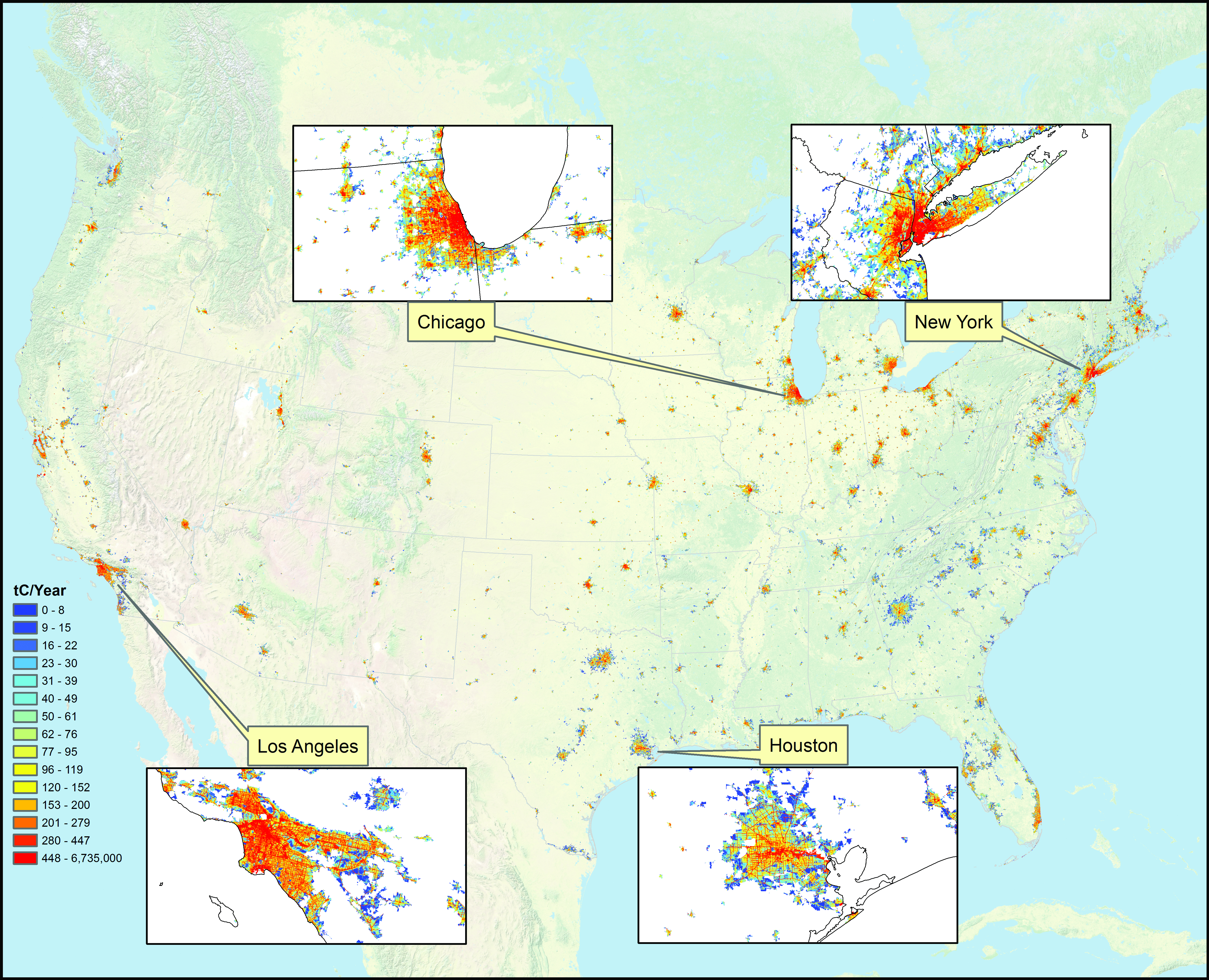
Figure 4.4: U.S. Fossil Fuel Carbon Emissions, Highlighting Four Urban Areas
Methane also is produced by municipal waste facilities. In Toronto, these facilities account for as much as 10% of urban emissions (City of Toronto 2013); in Indianapolis, about 35% of emissions are attributed to one landfill (Cambaliza et al., 2015; Lamb et al., 2016).
4.2.3 Land and Ecosystems
Urban development directly and indirectly alters above- and belowground vegetation carbon pools and fluxes through land clearing, removal of vegetation, and disruption of soils (Raciti et al., 2012). Estimates of urban vegetation carbon densities vary substantially among cities or states and are based on extrapolation of limited, nonrandom sampling. Using extensive remote sensors and field observations, case studies in both Maryland and Massachusetts found that developed areas hold about 25% of the biomass per unit area of nearby forests (Huang et al., 2015; Raciti et al., 2014). Trees in urban areas in the United States and Canada store an estimated 643 teragrams of carbon (Tg C) and 34 Tg C, respectively (Nowak et al., 2013). In contrast, studies in xeric ecosystems show relative enhancement in urban biomass densities that result from landscaping preferences and addition of non-native vegetation (McHale et al., 2017).
Growing conditions for vegetation in urban areas typically differ from nonurban ecosystems, potentially accelerating the cycling of carbon and nutrients (Briber et al., 2015; Reinmann and Hutyra 2017; Zhao et al., 2016). For example, urban areas experience elevated ambient air temperatures (i.e., the “urban heat island” [UHI] effect; Oke 1982). These elevated temperatures cause seasonally dependent changes in carbon fluxes from urban vegetation and soils (Decina et al., 2016; Pataki et al., 2006; Zhang et al., 2004; Zhao et al., 2016), altering the length of the urban growing season (Melaas et al., 2016; Zhang et al., 2006). Urban respiration and growth patterns also may differ due to human additions of water and fertilizers, removal or addition of labile carbon sources (e.g., leaf litter and mulch), and planting preferences (Templer et al., 2015). Urban vegetation also can influence local climate and energy use (Abdollahi et al., 2000; Gill et al., 2007; Lal and Augustin 2012; Nowak and Greenfield 2010; Wilby and Perry 2006). For example, urban trees may affect building energy consumption and associated carbon emissions directly through shading of building surfaces and altered use of cooling equipment (Raji et al., 2015) and indirectly through local reductions in air temperature (Nowak 1993; Sailor 1998). These effects require accounting for water and energy penalties associated with irrigation of managed urban vegetation (Litvak et al., 2017). In addition, fertilization of urban landscapes and management practices such as lawn mowing can carry a high energy cost that must be assessed when determining the net effect of urban vegetation on the carbon cycle (McPherson et al., 2005; Townsend-Small and Czimczik 2010).
See Full Chapter & References