Carbon Cycle Science in Support of Decision Making

Assuming adequate organization, communication, and funding is in place, there are a number of scientific and technical challenges associated with better connecting basic and applied science for decision-making purposes. This section discusses current capabilities and needs for data, modeling, accounting, and broad system approaches for carbon management.

18.4.1 Data Collection, Synthesis, and Analysis

Data for basic carbon research and decision making are often similar, although they typically are used independently instead of informing one another. For example, global climate models rely on national and global datasets on human activities and land management. Conversely, models of natural resource ecosystems and economics that inform land management require input on global changes in total land resources, commodity markets, and climate. A revised assessment of existing data, across disciplines, could help basic and use-inspired research on carbon and also address interrelated climate and carbon research issues.

Inventory data on fossil fuel emissions and land emissions and sinks are estimated nationally (e.g., U.S. EPA 2016) and reported internationally under the United Nations Framework Convention on Climate Change (UNFCCC). Advances in carbon cycle science are reflected in carbon modeling and accounting used to produce the inventory data. For example, field experiments that collect data on fertilizer application methods and timing, livestock and manure management, soil management, and other activities can be incorporated into models that estimate GHG emissions, thereby refining the national carbon budget.

Inventory data provide information on emissions sources and sinks and how net emissions change with land management or fuel supplies. To be most useful for local and regional planning, these data often require spatial distribution (West et al., 2014) or additional information on land-cover, land-use, and ecosystem characteristics that may be provided by satellite remote-sensing or economic survey data. Integrating inventory and remote-sensing data can provide new data products to understand local and regional carbon dynamics (Huang et al., 2015) and to inform land-management and policy decisions. Using integrated data on land use and management in climate modeling activities may become increasingly important (Hurtt et al., 2011) to facilitate consideration of climate feedbacks in local and regional decision making.

Although inventory data often serve as the basis for understanding human-induced impacts on the carbon cycle and subsequent decision making on carbon mitigation strategies, other datasets can provide additional or complementary estimates. For example, fossil fuel emissions can be estimated by the production of fossil fuels (U.S. EPA 2016) or by the consumption of fossil fuels (Patarasuk et al., 2016). The same is true for land-based emissions, which can be estimated using ground-level survey data from the Forest Inventory Analysis or the National Agricultural Statistics Service (West et al., 2011) or using atmospheric concentration data and modeled with atmospheric transport and inversion models (Schuh et al., 2013). The survey or inventory data represent “bottom-up” estimates while the atmospheric data represent a “top-down” approach. Reconciling data and approaches benefits both basic and applied science. Earth System Models (ESMs) require accurate base-level data and also need multiple ways to evaluate results. Similarly, inventory data used in models for decision making could benefit from alternative estimation approaches that evaluate existing inventory estimates (Jacob et al., 2016). Also needed are continued development and reconciling of data collection and modeling approaches to estimate carbon stocks and fluxes, requiring coordination among researchers, decision makers, and funding sources (see Box 18.1, Key Data Needs for Decision Making on Terrestrial Carbon).

18.4.2 Decision Support Tools for Carbon and Greenhouse Gas Management

Research models and decision support tools that can forecast future changes, as well as integrate and analyze current and past conditions, can provide solutions to challenges presented by climate change. At the broadest level, capabilities include assessment and decision-making tools that analyze feedbacks between human activities and the global carbon cycle. These capabilities can enable decision makers to 1) assess how changes in the carbon cycle will affect human activities and the ecosystems on which they depend and 2) evaluate how human activities—past, present, and future—impact the carbon cycle.

National GHG Inventories Critical for Modeling

For national-scale planning and in international agreements and negotiations, national GHG inventories have consistently been recognized as essential parts of the model-data system. Policy developments of the past few years have reinforced the global recognition of the need for high-quality and regularly reported GHG inventories. Increasing numbers of developing (i.e., UNFCCC non-Annex 1) countries produce annual GHG inventories and submit them to the UNFCCC using an extensive set of guidelines for national GHG reporting based on IPCC GHG inventory reporting guidelines (IPCC 1996, 2003, 2006). Deforestation and forest degradation constitute a major source of carbon emissions in many developing countries; the Global Forest Observations Initiative (GFOI) has developed guidance for using remotely sensed and ground-based data for forest monitoring and reporting of reduced emissions from deforestation, forest degradation, and associated activities produced in cooperation with UN-REDD and Forest Carbon Partnership Facility (FCPF) initiatives (http://www.gfoi.org/methods-guidance).

Most GHG inventories rest on estimates of the emissions associated with a particular activity (e.g., amount of CO₂ emitted per amount of fuel combusted). The factors that relate activities to emissions are called emissions factors. For sectors dominated by fossil fuels (e.g., power generation, transportation, and manufacturing), emissions factors are well constrained (IPCC 2006). Therefore, the major limitation to estimating emissions accurately is the ability to collect, organize, and verify the activity data (e.g., numbers of transformers upgraded, hectares of perennial plants established for bioenergy, and number of cattle raised on forage known to reduce CH₄ production). For biogenic-driven GHG emissions, such as those associated with agriculture and forestry, there is much greater variability in the emissions rate per unit of activity (e.g., N₂O emissions per unit of fertilizer added) because of heterogeneity in climate and soil conditions and in management practices. Dynamic process-based models offer an alternative approach that can account for this heterogeneity (Del Grosso et al., 2002; Li 2007), but using these models requires sufficient capacity (e.g., trained staff, functioning institutions).

GHG inventories that use activity data and emissions factors (or activity-specific process modeling) are referred to as bottom-up approaches (see Section 18.4.1). All national GHG inventories use this approach, which, by definition, attributes emissions sources and sinks to identifiable entities and activities and lends itself to policy applications to reduce emissions and incentivize sinks. Examples of spatially explicit, high-resolution model-data systems for major source categories include fossil fuel emissions (Gurney et al., 2012; Gurney et al., 2009), forest dynamics (USDA 2015), biofuels (Frank et al., 2011), and land-use change (Sleeter et al., 2012; Woodall et al., 2015). These data combine knowledge of biophysical processes with data on human activities and economics that can help municipalities or geopolitical regions understand and quantify carbon emissions and sinks, thereby informing decision making. Challenges to these bottom-up approaches, aside from improving data quality on both activities and emissions factors to reduce uncertainties, include ensuring completeness and avoiding double-counting of sources.

Land-Use Emissions Projections and Examples of Sector-Specific Tools

In addition to inventories, the carbon cycle science community develops projections that scale from local mitigation options to global impacts and, conversely, from global economic forces to local strategies. Many countries incorporate land-use emissions into their overall climate targets in some way, and these projections inform national and international strategies to address CO₂ emissions, carbon management options, and other sustainability goals. These estimates of future land-use sources and sinks are useful for decision making because they stem from a reliable, scientifically sound, and transparent process (U.S. Department of State 2016). Because this work reflects the development and use of new approaches in carbon cycle science, further work is widely acknowledged as being helpful to increasing the usefulness of land-use emissions projections.

Models and decision tools have also been designed to help industry, business, or other entities (e.g., universities, land-management agencies, farmers, and ranchers) assess their emissions and develop mitigation strategies. In a regulatory environment where emissions are in some way limited by law, models and decision tools are essential for planning, forecasting, and monitoring emissions reductions. These tools also are widely used in voluntary carbon accounting and reporting to generate and sell carbon credits from a variety of activities (CARB 2018).

Models and decision support tools for inventory and forecasting in the AFOLU sector at the scale of the farm, woodlot, or business have been developed and are increasingly deployed as tools to guide implementation of government-sponsored conservation programs. These tools can help inform decisions to reduce the GHG footprint of agricultural commodities through supply-chain management by agricultural industries and to support agricultural offsets in carbon cap-and-trade systems (see examples below).

• COMET-Farm (cometfarm.nrel.colostate.edu; Paustian et al., 2018)—Helps farmers and other landowners estimate carbon benefits associated with implementing practices supported by conservation programs of the USDA Natural Resources Conservation Service (Eve et al., 2014).

• Cool-Farm Tool (CFT; www.coolfarmtool.org/CoolFarmTool; Hillier et al., 2011)—A product of the Cool Farm Alliance, CFT is designed for use by farmers and is intended to support the Alliance’s global mission of enabling millions of growers to make more informed on-farm decisions that reduce their environmental impact.

• DNDC (Denitrification-Decomposition) process-based biogeochemical model (Li 2007)—Used by institutions like the California Air Resources Board to support CH₄ reductions from rice farming as an agricultural GHG offset in California’s GHG emissions reduction program (Haya et al., 2016).

• ExACT (Ex-Ante Carbon balance Tool; www.fao.org/tc/exact/ex-act-home/en)—Estimates CO₂ equivalent (CO₂e)² emissions based on a project’s implementation as compared to a “business-as-usual” scenario. Project designers can use ExACT as a planning tool to help prioritize mitigation-activity terms.

• ALU ( Agriculture and Land Use) national GHG inventory software—Assists countries in completing their national inventories. This tool was developed to meet a U.S. governmental priority of increasing the number of countries developing robust GHG inventories to create transparent, evidence-based understanding of global GHG emissions.

• Climate Change, Agriculture, and Food Security–Mitigation Options Tool ( CCAFS–MOT)—Identifies practices in Africa, Asia, and Latin America that can reduce emissions and sequester carbon on agricultural lands. MOT prioritizes effective mitigation options for many different crops according to mitigation potential, considering current management practices, climate, and soil characteristics.

• National Oceanic and Atmospheric Administration (NOAA) Annual Greenhouse Gas Index—Compares the total combined warming effects of GHGs (including CO₂, CH₄, N₂O, and chlorofluorocarbons) to their 1990 baseline levels.

• Bioenergy Atlas—Includes maps enabling the comparison of biomass feedstocks, biopower, and biofuels data from the U.S. Department of Energy (DOE), U.S. Environmental Protection Agency (EPA), and USDA. (Software hosted by DOE’s National Renewable Energy Laboratory.)

• Global Carbon Atlas—Aggregates global carbon data to explore, visualize, and interpret global and regional carbon information and changes from both human activities and natural processes. (Supported by the Global Carbon Project, www.globalcarbonproject.org; and BNP Paribas.)

Comparable decision support tools for carbon management have been developed for other sectors. For example, USAID’s Clean Energy Emissions Reduction (CLEER) tool, based on internationally accepted methodologies, enables users to calculate changes in GHG emissions resulting from adoption of geothermal; wind; hydroelectric and solar energy generation; upgrades of transmission and distribution systems; increases in building energy efficiency; heating, ventilation, and air conditioning system efficiency improvements; fuel switching; capture of stranded natural gas by flaring; use of biomass for energy; and use of anaerobic digesters to capture CH₄ from livestock manure (USAID 2018).

Complex, Multisector Modeling

Integrated Assessment Models merit particular attention because they constitute a distinct field of research and serve a unique role in decision support. Among decision support tools for carbon management, IAMs are unique in estimating economy-wide responses, including GHG emissions, to different management and policy options. The objective of these models is to capture the primary interactions and interdependencies between natural and human systems (e.g., economic sectors) through a series of scenarios that represent plausible policy interventions (Weyent 2017). These models can help understand feedbacks among carbon sources and sinks at national and global scales (see Figure 18.3), given specified emissions targets or implementation of carbon strategies (Grassi et al., 2017; Iyer et al., 2015). Integrative modeling frameworks that include land sector, energy sector, transportation, and other interconnected carbon sources and sinks have continued to develop more detailed model structures and higher-resolution data input (Kyle et al., 2011; Wise et al., 2014).

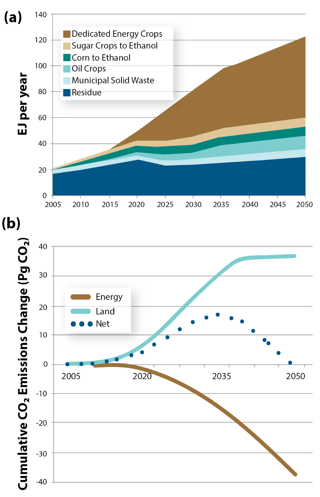
IAMs, designed to answer questions about carbon management, include 1) social and economic factors that drive GHG emissions as well as a representation of biogeochemical cycles that determine the fate of those emissions and 2) the effects on climate and human welfare. The dynamic interactions among sectors in these models mean that they can reveal nonintuitive outcomes. Actions in one sector or geography can influence those in another, and a common goal of carbon management policy is to limit the accumulation of CO₂ in the atmosphere. Therefore, understanding the economy-wide influences of policy choices is critical both to assess the actual consequences of a single policy on carbon accumulation in the atmosphere and to have a realistic idea of the level of atmospheric CO₂ that could be achieved with multiple countries and multiple policies.

Continued efforts to integrate IAMs, ESMs, carbon accounting, and national-scale resource modeling will help develop consistency in data input across these modeling platforms. The combination of global IAMs, national and subnational natural resource economic models, carbon accounting methods, land-use change models, energy technology, and market analyses are all needed to estimate carbon management strategies in a comprehensive manner from the local to global scale (see Box 18.2, Carbon Modeling Needs for Decision Making). As one example, a process using IAMs, global and national natural resource (i.e., timber) models, and inventory data (i.e., field surveys) was conducted in the development of the United States Mid-Century Strategy for Deep Decarbonization (White House 2016).

18.4.3 Carbon and Greenhouse Gas Accounting

Data and models that estimate changes in carbon flux often were not initially developed for estimating direct and indirect net carbon changes associated with given activities. This is true for country-level inventory data reported by sector (U.S. EPA 2016), biogeochemical cycle models (Del Grosso et al., 2002), and integrated climate models (Wise et al., 2009). In many cases, incorporating the influence of particular activities on upstream or downstream energy, land use, and associated GHG emissions significantly changes estimates of the realized carbon savings. Full GHG accounting of all emissions related to a given activity can significantly augment or reduce reported emissions compared to partial or incomplete accounting.

Accounting of carbon fluxes and stock changes in ecosystems or industrial systems dates back to early work on energy input and output models and systems modeling (Odum 1994) and has evolved rapidly since then. A systems analysis can be developed to understand and quantify net carbon exchange associated with specific management activities (Schlamadinger and Marland 1996). Such analyses, for example, consider disturbance (e.g., widespread tree mortality and erosion from hurricanes or ice storms), forest regrowth over time, landscape area boundary, and forest growth trends over time in the absence of disturbance (Lippke et al., 2011; Lippke et al., 2012). Fossil fuel offsets associated with harvested wood and wood products are also included in these system-scale carbon budgets. These types of analyses often are conducted to illustrate the methods and provide an averaged national answer. To be useful for decision making, full carbon accounting would need to be conducted for regions that have obvious differences in ecosystem attributes, climate regimes, and social and economic drivers (see Box 18.3, Carbon Accounting Needs for Informing Decision Making).

Past development of carbon accounting methods suggests a number of basic carbon accounting guidelines. Properly defining time and space boundaries of the system or activity of interest is an essential first step, and highlighted below are additional guidelines.

Stock Changes Are Less Prone to Error than Adding up All Biological Fluxes and Uptakes. This finding is currently guiding analyses by EPA’s Science Advisory Board Panel on Biogenic Emissions from Stationary Sources on net carbon emissions from the use of biomass for energy production (U.S. EPA 2014). The stock change approach also has been the chosen method for estimating net emissions from forests and agricultural soils (U.S. EPA 2016). Trying to simulate all fluxes in and out of a system is useful for understanding ecosystem processes and climate feedbacks, but the increased complexity may introduce additional error and uncertainty. In contrast, changes in carbon stocks inherently combine the net result of multiple fluxes into and out of a given stock entity. Differences in complex models and stock change methods are exemplified in an analysis by Hayes et al. (2012).

Accounting for Energy and Emissions One-Level Upstream and Downstream Is Often Sufficient to Capture Adequately the Total Flux Associated with an Activity of Interest. When estimating emissions associated with changes in fertilizer application rates, for example, the fuels used to process the fertilizer (e.g., natural gas) should be considered (i.e., Level 1 upstream), but the energy used to mine the fuel (e.g., natural gas; Level 2 upstream) is often statistically insignificant (West and Marland 2002). Although exceptions should always be considered, accounting for emissions of both Level 1 upstream and downstream (e.g., transporting the fuel) of the activity of interest remains a good general rule.

Establishing the Proper Reference Point (System that Exists Prior to Changes in Management) Is Essential. The reference point is the current system, prior to a change in activity (see Figure 18.4). The reference point should not be chosen at a time prior to the current activity (e.g., based on historical trends), nor should it be arbitrarily chosen before or after activities associated with the new or alternative management. This issue is currently debated in regard to some forest management techniques (Campbell et al., 2012; Hurteau and North 2009).

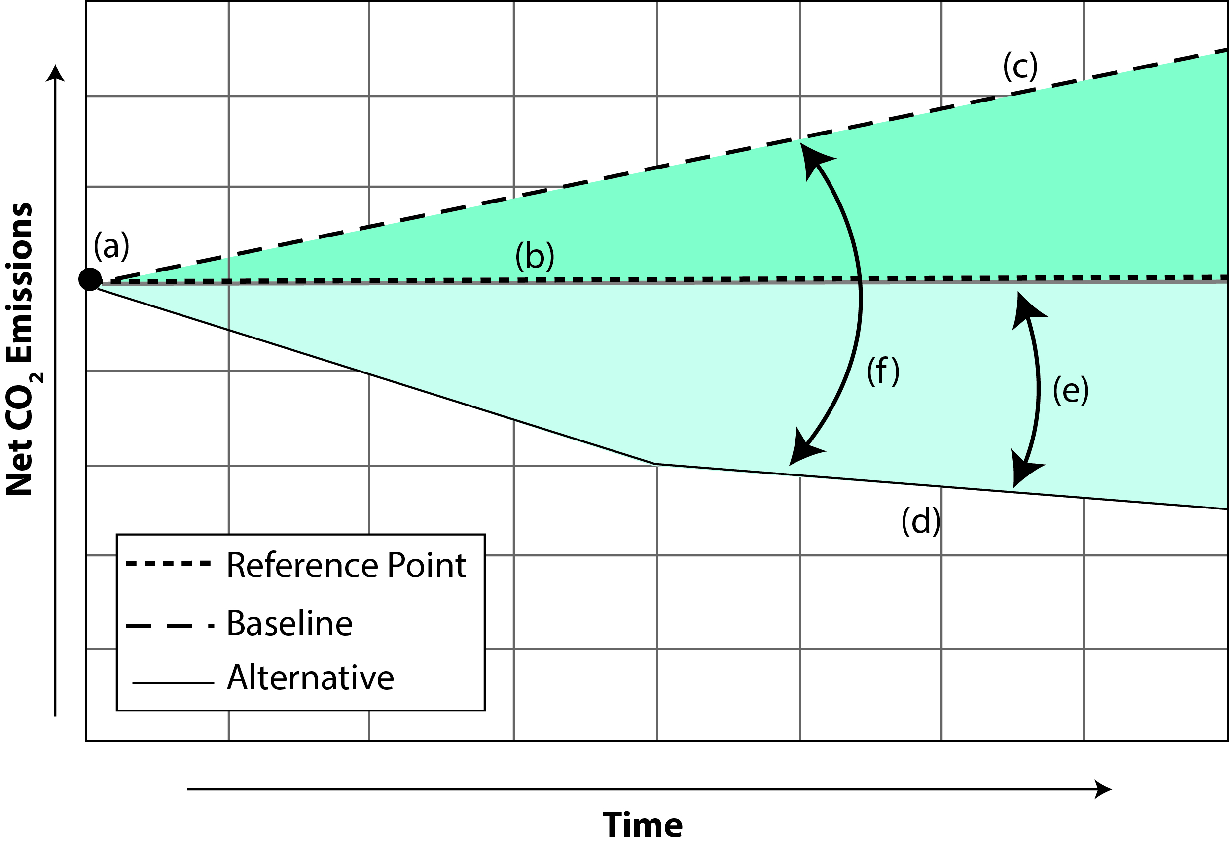
A Baseline Trajectory May Be Conceptually More Comprehensive Than a Reference Point But May Have More Uncertainty. Models that project changes in land use, fossil fuel combustion, or other GHG emissions can be particularly useful for understanding future scenarios. However, the trend line for the future trajectory can be uncertain, and using baselines to compare new or alternative systems should only be done with caution (Buchholz et al., 2014). The use of a reference point or baseline should be decided based on the certainty associated with baseline projections (see Figure 18.4). For example, a baseline of forest growth (e.g., increased growth until forest maturation) is well established in forest growth curves, whereas future changes in land use based on commodity markets is less certain. There may also be policy considerations that influence whether baselines or reference points are more appropriate for a given context.

18.4.4 Systems Approach for Decision Making

Combining several of the aforementioned capabilities (e.g., data collection, modeling, and accounting) can help facilitate the use of research products for both decision making and the next generation of new relevant scientific analyses (West et al., 2013). Data assimilation systems have been under development to bring together inventory-based datasets, atmospheric modeling, global land models, and accounting procedures. Integrating these research areas using data assimilation, where appropriate, can help researchers explore data similarities and differences, reconcile data differences, and potentially integrate datasets to attain enhanced data products or model results with reduced bias, reduced uncertainty, and improved agreement with observations. Past efforts include 1) a project in the midwestern United States (Ogle et al., 2006), 2) a North American continental analysis (Hayes et al., 2012; Huntzinger et al., 2012), and 3) similar analyses in Europe (Le Quéré et al., 2015). Of these analyses, those for the midwestern United States and Europe resulted in little to no statistical difference between bottom-up and top-down emissions estimates, indicating promising capability in using one method to constrain another and in integrating methods for a more comprehensive and potentially more accurate estimate. There also is an indication that atmospheric inversion model estimates (i.e., top-down estimates) can be useful in smaller regions, but they are potentially less informative or accurate at continental or global scales (Lauvaux et al., 2012). Accounting issues also were identified and resolved between atmospheric estimates and terrestrial-based estimates so that the two methods could be compared and contrasted, contributing to a new lexicon that helped define land-based fluxes in a manner consistent with fluxes observed from atmospheric measurements (Chapin et al., 2006; Hayes and Turner 2012).

Although reconciling bottom-up and top-down estimates can help build confidence in existing estimates, thereby forming a stronger foundation for decision making, other existing modeling systems could be combined to improve national and global decision making about carbon. Largely independent efforts continue for climate modeling, land-use modeling, global and regional economic modeling, and energy modeling. Coordinating these modeling activities so that, at a minimum, output from one model can be used as input for other models would help in coordinating decisions that inherently affect or are affected by climate, land use, and energy production and consumption (see Figure 18.1). This effort would require high-level coordination among research organizations that support modeling in different research fields covering fundamental, applied, and social sciences (see Box 18.4, Research Needs for Integrative Observation and Monitoring Systems).